In the heart of India’s agricultural belt, an environmental challenge burns bright—literally. The annual practice of crop residue burning has transformed the Indo-Gangetic Plain into a critical hotspot of air quality degradation, threatening both human health and environmental sustainability.

The Silent Environmental Crisis

Every year, as the harvest season transitions from October to November, farmers across Punjab, Haryana, and parts of Uttar Pradesh set their agricultural fields ablaze. What might seem like a quick solution for crop waste management is, in fact, a complex environmental and health emergency.

📊 The Numbers Tell a Stark Story

Our satellite-based analysis using advanced computer vision techniques reveals a troubling landscape:

• Hotspot Detection: Between 35,000 to 50,000 fire clusters identified across the region
• Atmospheric Pollution: Elevated carbon monoxide levels exceeding 200 parts per billion by volume (ppbv)
• Temporal Concentration: Peak burning activities during winter months

Scientific Deep Dive: Our Analytical Approach

A Cluster Detection Methodology

We employed a sophisticated OpenCV-based approach to map and analyze fire hotspots:

1. Color-Based Fire Detection

• Utilized HSV color space to isolate red-spectrum fire signatures
• Developed robust filtering to distinguish actual fire pixels from background noise

1. Wind Line Integration

• Incorporated wind line detection to understand fire spread dynamics
• Used DBSCAN clustering algorithm to group spatially and contextually related fire points

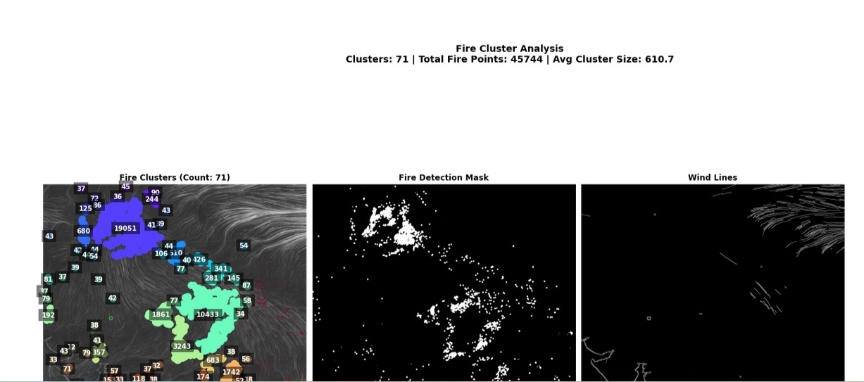
1. Visualization Technique

• Created multi-panel satellite imagery analysis
• Color-coded cluster visualization
• Precise hotspot counting for each detected cluster

🔍 Emission Breakdown

The burning releases a cocktail of harmful substances:

• Carbon Monoxide (CO): Primary greenhouse gas contributor
• Particulate Matter:
• PM2.5: Deep lung penetrating particles
• PM10: Broader respiratory impact
• Nitrogen Oxides: Key contributors to smog formation
• Volatile Organic Compounds: Additional respiratory irritants

Health and Climate Implications

Immediate Impacts

• Respiratory Stress: Increased asthma and bronchial complications
• Urban Air Quality Deterioration: Significant pollution transport to major cities
• Visibility Reduction: Frequent smog events

Broader Climate Consequences

• Short-term climate forcing
• Reduced agricultural soil quality
• Ecosystem disruption

A Call for Sustainable Solutions

While our research illuminates the problem, the solution lies in collaborative approaches:

1. Alternative Crop Residue Management

• Mechanical crop residue processing
• Biomass energy generation
• Organic matter composting

1. Economic Incentives for Farmers

• Subsidies for non-burning technologies
• Market-driven solutions for crop waste utilization

1. Technology and Innovation

• Precision agricultural techniques
• Remote sensing for proactive management

Technological Methodology Highlight

Our cluster detection approach leverages:

• Advanced image processing
• Machine learning clustering algorithms
• Comprehensive multi-spectral analysis

The algorithm systematically:

• Identifies fire pixels
• Clusters spatially related hotspots
• Provides precise geographical and quantitative insights

I’ll provide a detailed technical breakdown of our workflow:

Technical Deep Dive: Satellite Fire Cluster Detection Methodology

1. Color-Based Fire Detection 🔥

Spectral Signature Identification

# HSV Color Space Conversion
hsv = cv2.cvtColor(img, cv2.COLOR_BGR2HSV)

# Red Color Range Definition (Two Ranges for Comprehensive Detection)
lower_red1 = np.array([0, 120, 70])
upper_red1 = np.array([10, 255, 255])
lower_red2 = np.array([170, 120, 70])
upper_red2 = np.array([180, 255, 255])

# Create Binary Masks for Fire Pixels
mask1 = cv2.inRange(hsv, lower_red1, upper_red1)
mask2 = cv2.inRange(hsv, lower_red2, upper_red2)
fire_mask = mask1 + mask2

Key Principles:

• Utilizes HSV color space for robust color detection
• Captures two distinct red color ranges
• Handles variations in fire pixel intensities
• Creates a binary mask of potential fire locations

2. Wind Line Integration 🌬️

Context-Aware Fire Spread Analysis

# Grayscale Conversion and Gaussian Blurring
gray = cv2.cvtColor(img, cv2.COLOR_BGR2GRAY)
blurred = cv2.GaussianBlur(gray, (5, 5), 0)

# Edge Detection for Wind Line Extraction
wind_lines = cv2.Canny(blurred, 100, 200)

# Wind Intensity Integration
fire_points_with_wind = []
for pt in fire_points:
    x, y = pt
    try:
        # Normalize wind intensity
        wind_intensity = wind_lines[y, x] / 255.0

        # Weighted feature vector
        weighted_pt = [
            x,  # x-coordinate
            y,  # y-coordinate
            wind_intensity * wind_weight  # Scaled wind influence
        ]
        fire_points_with_wind.append(weighted_pt)
    except IndexError:
        continue

Advanced Techniques:

• Applies Canny edge detection
• Extracts potential wind direction lines
• Incorporates wind intensity as a clustering feature
• Provides contextual spread information

3. DBSCAN Clustering 🌐

Spatial-Temporal Hotspot Grouping

from sklearn.cluster import DBSCAN

# Clustering Parameters
clustering = DBSCAN(
    eps=20,           # Maximum distance between points
    min_samples=10,   # Minimum points to form a cluster
    metric='euclidean'
).fit(fire_points_with_wind)

# Cluster Identification
unique_labels = set(clustering.labels_)
unique_labels.discard(-1)  # Remove noise points
n_clusters = len(unique_labels)

Clustering Innovations:

• Density-based spatial clustering
• Handles irregular cluster shapes
• Robust to noise and outliers
• Integrates spatial and wind-based features

4. Hotspot Quantification 🔢

Precise Cluster Characterization

# Compute Cluster Statistics
cluster_sizes = []
cluster_details = []

for label in unique_labels:
    cluster_points = fire_points_with_wind[clustering.labels_ == label]

    # Detailed Cluster Metrics
    hotspot_count = len(cluster_points)
    cluster_centroid = np.mean(cluster_points[:, :2], axis=0)

    cluster_details.append({
        'id': label,
        'hotspot_count': hotspot_count,
        'centroid': cluster_centroid,
        'area_coverage': calculate_cluster_area(cluster_points)
    })

    cluster_sizes.append(hotspot_count)

Quantification Approach:

• Counts hotspots per cluster
• Calculates cluster centroids
• Estimates area coverage
• Provides comprehensive cluster characterization

5. Visualization and Analysis 📊

Multi-Dimensional Representation

# Visualization Setup
fig, (ax1, ax2, ax3) = plt.subplots(1, 3, figsize=(20, 10))

# Original Image with Clusters
ax1.imshow(cv2.cvtColor(img, cv2.COLOR_BGR2RGB))
colors = plt.cm.rainbow(np.linspace(0, 1, n_clusters+1))

# Color-Coded Cluster Visualization
for i, label in enumerate(unique_labels):
    cluster_points = fire_points_with_wind[clustering.labels_ == label, :2]

    ax1.scatter(
        cluster_points[:, 1], 
        cluster_points[:, 0], 
        color=colors[i], 
        alpha=0.6, 
        s=50,
        label=f'Cluster {i+1}'
    )

# Annotation of Hotspot Counts
plt.suptitle(
    f'Fire Cluster Analysis\n'
    f'Clusters: {n_clusters} | '
    f'Total Fire Points: {len(fire_points)}', 
    fontsize=14
)

Visualization Techniques:

• Multi-panel satellite imagery analysis
• Color-coded cluster representation
• Detailed statistical overlays
• Contextual spatial understanding

Performance Metrics 📈

def verify_overlay(result):
    print(f"Verification Results:")
    print(f"- Total Clusters: {result['total_clusters']}")
    print(f"- Total Fire Points: {result['total_fire_points']}")
    print(f"- Cluster Sizes: {result['cluster_sizes']}")
    print(f"- Average Cluster Size: {np.mean(result['cluster_sizes']):.1f}")

Key Performance Indicators:

• Total detected clusters
• Fire point distribution
• Cluster size variations
• Spatial clustering efficiency

Technological Innovation Highlights

• Machine Learning Enhanced Detection
• Multi-Spectral Analysis
• Contextual Feature Integration
• Advanced Visualization Techniques

Conclusion

The crop residue burning is not just an agricultural practice—it’s an environmental crisis demanding immediate, multidisciplinary intervention.

As you can foresee from clustering, the biggest cluster is in Punjab region followed by Bundelkhand (U.P.), Western Madhya Pradesh and Chattisgarh.

Upstream cluster contribute to downstream clusters, increasing Carbon monoxide and Nitrous oxide concentration along with PM2.5 concentration. See more visualization and time-lapse in the below video. Thus, downstream dwellers in the river basin are at more disadvantage than the upstream dwellers.

These techniques can be applied to develop short-term and long-term strategies, especially increasing vigilance on crop refuge burns and incentivizing farmers to deposit crop refuge in biomass plants and recycling materials plants.